What is remote sensing?

Remote sensing is often defined as acquiring information about objects without being in direct physical contact with them. Our ears, eyes, and cameras are examples of remote sensors. More specifically, remote sensing is the science of collecting and interpreting electromagnetic information about the earth using sensors on platforms in our atmosphere (balloons, airplanes) or in space (satellites).

The electromagnetic spectrum

The electromagnetic (EM) spectrum describes a continuous spectrum of energy.  This energy is caused by the movement of electrical charges. Visible light, or the light that our eyes can detect, is just a small portion of the EM spectrum.  Using specialized sensors, we can look into the realm of the invisible and see a greater portion of the EM spectrum than is possible with the human eye.

Almost all EM energy surrounding us is produced by the Sun. Sunlight that travels through space and shines on the Earth is termed "solar radiation."  This energy can be absorbed, transmitted (passed through), scattered, or reflected by particles in the atmosphere or objects on Earth.

Remote sensing of the electromagnetic spectrum

Electromagnetic radiation is the source of all signals collected by remote sensing instruments. The region of the EM spectrum that is measured depends on the sensor's characteristics. Sensors collect data by separating reflected portions of the EM spectrum into separate bands as shown in the figure below. Note that the image produced using one band is black-and-white, this is often called a "grayscale image."

Image structure

The image produced by sensor data is made up of one to several bands (the bands can be thought of as layers). These bands measure the intensity of reflected light from the specified regions of the EM spectrum.

Each band is composed of individual elements that are arranged in a grid of rows and columns. The individual elements are called “pixels”. The word “pixel” is derived from the term “picture element”. A pixel is the smallest unit of ground area measured by the sensor. Each pixel has a numerical value which corresponds to the amount of reflected light.

The number of bands and the size of the pixels differ from sensor to sensor.

Let’s look at a portion of the QuickBird image for Mākaha Valley. This image is made using three bands: the red, blue, and green bands. If we zoom into the area shown by the red box, the rows, columns, and pixels can be seen. Zoom in a lot more and we can see one pixel. QuickBird pixels are 2.4 m by 2.4 m.

As you look at the image on the far right, you can see pixels with different colors. How are the pixel's numerical values translated into color on the computer?

In computers, color is produced on screens using combinations of red, green, and blue (usually abbreviated as RGB). In order to magnify the reflectance intensities in remotely sensed data, and also to see regions of the EM spectrum undetectable to human eyes, grayscale images are displayed by assigning them to one of these color filters.

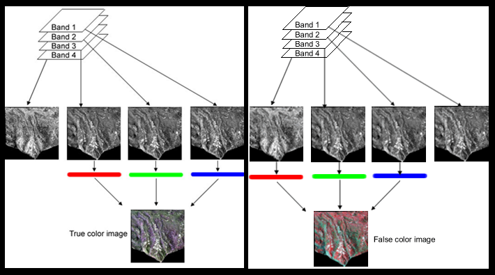
In order to see an image the way our eyes would normally see it, we would assign the red band to a red filter, the green band to a green filter, and the blue band to a blue filter. This band and color combination produced a "True Color Image." However, it is sometimes useful to assign bands to unusual color filters, thus producing a "False Color Image." For example, if we assign the near-infrared (NIR) band to red, the red band to green, and the green band to blue, we produce a commonly used combination used to study vegetation. Vegetation is characterized by low red reflectance and very high NIR reflectance. Adding the NIR band to an image display helps to distinguish vegetation zones.

Below, almost everything is green in the true color image on the left (although subtle variations in the color are noticeable). In the false color image on the right, it is easier to see vegetation with higher reflectance. These high reflectance areas are red. Vegetation with lower reflectance in the false color image is green. Choosing how remotely sensed data are displayed on the computer aids tremendously in understanding land cover classes.

Image classification

When we classify the image data, it is most helpful if we analyze the pixel values in addition to observing image color and texture. This is one of the big advantages that images have over photographs. Each pixel contains a value which can be quantitatively manipulated and analyzed using computer software.

As an example, say that you were to look at two different pixels. In a true color image, one pixel is brown and the other pixel is green. In a false color image, the brown pixel appears blue and the green pixel appears red. Based on this information, you might be able to guess what kinds of material are causing the two different reflectance values. However, another way to classify the pixel would be to look at its spectral profile. The spectral profile is obtained by graphing the pixel values (reflectance) for the different bands.

Beneath the pixels below, there are two graphs. Compare the shape of these two graphs to the graph in the lower right corner. For this particular satellite (IKONOS), we are getting information from the blue, green, red, and NIR regions of the EM spectrum. So, compare the spectral profiles for the two pixels to the area outlined in gray. The spectra in this graph are representatives of typical soil, water, and vegetation spectra. The quantitative data provide strong evidence that the brown/blue pixel is soil and the green/red pixel is vegetation.

Computer software can statistically analyze the quantitative data, group similar pixels, and separate dissimilar pixels. Two general types of algorithms are available, "supervised" and "unsupervised."

In supervised classification, pre-determined landcover classes are defined, and their spectral characteristics are extracted from representative pixels in an image. These areas are known as the "training areas". The entire image is then analyzed by comparing each pixel's reflectance to the reflectance of the training areas.

In unsupervised classification, the computer program first groups pixels in the image into statistically separate clusters, depending on their reflectance values. The desired level of separation (the number of classes and their degree of separability) is specified by the analyst, who must eventually assign a meaningful landcover class.

It is important to correlate remotely sensed map classes to detectable differences in ground classes. Once correlation is complete and a map is produced, additional field information is needed to assess the accuracy of the map.

Sensor characteristics

As we have seen above, different sensors have different characteristics. These characteristics are based on expected usage and technological limitations. It is important to choose the appropriate sensor data based on project needs. In the table below, spectral bands and their spatial resolutions are given for each of our studied sensors.

* ASTER produces 5 bands in the SWIR 2 region.

This information and some of the figures were compiled from the: American Museum of Natural History's Biodiversity Informatics Facility, Aster User Handbook, Dundee Satellite Receiving Station, GeoEye, NASA's Landsat Program, Satellite Imaging Corp, USGS Landsat Website